
Policy Gradients in a Nutshell?!
If you are not familiar with the foundations of reinforcement learning then you should check one of these pages: Open AI’s page, Lilian Wang’s blog
Introduction
In a nutshell, Policy Gradient (PG) methods are part of the reinforcement learning family where the agent learns the policy directly. There are value-based methods (VB) where the agent learns the value of certain action on a certain state, and it chooses the action with the maximum value over the other actions. In PG you don’t calculate any state or state-action value, the agent learns directly the policy based on the value of the reward. It increases or decreases the certain action probability and of course, it pushes the other available action probabilities to the opposite direction. Let’s clarify with an example: the environment is a grid table and there are 4 available actions (up, left, right, down) and you randomly choose different states on this surface. After taking 4 steps you can’t move further because you have reached a terminal state, and let’s assume that one is the goal state and you get a reward which is 10. You wrote down every state’s names and the actions that you chose and of course, you also know the value of the reward which was positive, so you conclude that your choice can be a good path and you should follow it in the future. This is a very simple but valid example if the environment is discrete, but life is more complex than this (even Super Mario).
As I mentioned above in the introduction: VBs learn the policy indirectly (it learns the action-state values and map a policy from it).
Formally: \(\pi(s) = argmax_a Q(s,a)\).
In contrast, policy-based methods learn the policies directly, which can be more efficient in many cases rather than calculating the value of the action over all the other actions. For instance, in an environment that contains high-dimensional or continuous action spaces.
Another big advantage is that policy-based approaches can learn stochastic policies, which make sense in many cases, think about a partially observable environment (e.g: the foggy lake) or in non-cooperative games (Nash equilibrium e.g: rock-paper-scissors).
Stochastic policy formally: \(\pi(s,a) = \max_{\pi}\mathbb{E}[G \mid \pi]\)
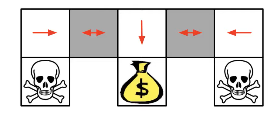
A really good example for stochastic policies: DeepMind X UCB, Stanford CS234. This simple environment contains 3 terminal states (2 skull heads, and one bag of gold) where the agent’s goal is to find the bag of gold as fast as she can. The grey states are special, the agent isn’t able to distinguish them. If the policy is deterministic then she always steps in the left or the right direction on these special states, which means she will get stuck on the side of the board.
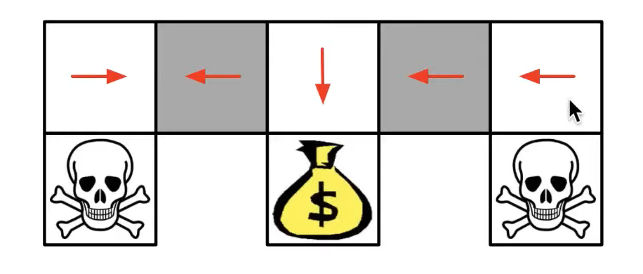
The best she can do on those states is sampling randomly between left and right actions. This is a perfect example of when stochasticity is necessary to reach the maximum returns.
Policy optimization
As you can see, this is an optimization problem and we have to calculate the performance of the actual parameters \(\theta\) of the function approximator \(\pi\) and iteratively increase the probability of the good actions and decrease the bad ones, because this maximizes the expected returns \(G\).
But how are we gonna optimize the parameters based on the returns?
Returns are numbers which means we can’t differentiate them.
There is a gradient estimation technique Score Function Gradient Estimator or Log-Likelihood Ratio Gradient Estimator which can help us to fix this issue.
But before we start differentiating the equation we should clarify what is the learning objective which must be different based on the type of the environment.
Episodic environment: average reward per episode.
Continues environment: average reward per step.
Formally:
\(J(\pi_\theta) = \mathbb{E}_{\tau \sim \pi_\theta}[G(\tau)]\)
Note \(\tau\) (tau) is the trajectory.
Also the way to update the parameters:
\(\theta_{e+1} = \theta_e + \alpha * \nabla_\theta J(\pi_\theta)\)
Where \(\theta\) is the parameters of the policy \(e\) is the current episode (or the current batch), \(\alpha\) is the learning rate of the gradient ascent and \(\nabla_\theta J(\pi_\theta)\) is the gradient of our policy. In supervised learning we use gradient descent since we want to minimize the difference between the predicted and the true labels. In PG world we try to maximize the expected returns, this is why we use the gradient ascent, we want to reinforce the good trajectories \(\tau\) and punish the bad ones.
Deriving the policy
As I mentioned above we estimate the gradients of the expectations w.r.t the parameters.
A couple of notations:
Trajectory contains states, actions, rewards from the sampled episode(s).
\(\tau = s_0, a_0, r_1, s_1, a_2 ... s_{T-1}, a_{T-1}, r_T, s_T\)
Returns (in this case discounted returns)
\(G(\tau) = r_1 + \gamma r_2 + \gamma^2 r_3 ... \gamma^{T-1} r_T\)
Probability of a trajectory (p0 is the initial state, Ps are the transition probabilities)
\(P(\tau \mid \theta) = p(s_0) \pi_{\theta}(a_0 \mid s_0) P(s_1,r_1 \mid s_0,a_0) \pi_{\theta}(a_1 \mid s_1;\pi) ... P(s_T,r_T \mid s_{T-1},a_{T-1})\)
Derivation
\(\nabla_\theta J(\pi_\theta) = \nabla_\theta \mathbb{E}_{\tau \sim \pi_\theta}[G(\tau)]\) # Definition of \(\nabla_\theta J(\pi_\theta)\) (1)
\(= \nabla_\theta\int_{\tau} P(\tau \mid \theta) G(\tau)\) # Expanded expectation (2)
\(= \int_{\tau} \nabla_\theta P(\tau \mid \theta) G(\tau)\) # Leibniz integral rule (swap \(\nabla\) & \(\int\)) (3)
\(= \int_{\tau} \frac{P(\tau \mid \theta)}{P(\tau \mid \theta)} \nabla_\theta P(\tau \mid \theta) G(\tau)\) # Multiply by 1 (Identity term 7.1 Example 6.) (4)
\(= \int_{\tau} P(\tau \mid \theta) \frac{\nabla_\theta P(\tau \mid \theta)}{P(\tau \mid \theta)} G(\tau)\) # Rearrange (5)
\(= \int_{\tau} P(\tau \mid \theta) \nabla_\theta log{P(\tau \mid \theta)} G(\tau)\) # \(\frac{\nabla f}{f} == \nabla log(f)\) (6)
\(= \mathbb{E}_{\tau \sim \pi_\theta} [\nabla_\theta log{P(\tau \mid \theta)} G(\tau)]\) # Rewrite as an expectation (7)
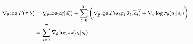
Above you can see the definiton of \(\nabla_\theta J(\pi_\theta)\) (1) that we are going to derive and as you can see we can rewrite it in an expanded form (2). At line (3) we use the Leibniz integral rule that allows us to exchange the order of integration and differentiation. At line (4) we multiply by 1, which is important because we need an expectation form again and thanks to this identity we can rearrange (5) and simplify the equation (6) and rewrite as an expectation (7). \(\nabla_\theta log{P(\tau \mid \theta)}\) contains the initial state and the transition probabilities that don’t depend on parameters \(\theta\), it means we can erase them from the equation. (Not neccessary to transform from \(\frac{\nabla f}{f}\) to \(\nabla log(f)\) but gradient calculations are numerically more stable in this way.)
There is a nice explanation on Open AI webpage (derivation also based on that article).
I don’t want to write everything that many other people did, so if you are interested in the proof of the Policy Gradient Theorem and would like to expand your knowledge about other interesting details I recommend you to read R. Sutton’s book (Chapter #13).
We can transform this form again, the way that we can take samples and repeatedly calculate the gradient and update the parameters of the policy.
\(\nabla_\theta J(\pi_\theta) = \frac{1}{N}\sum_{i=0}^N \nabla_\theta log \pi_ (\tau_i \mid \theta) * G(\tau_i )\)
There are interesting gradient-free policy solutions (e.g: evolution strategies): Malik et al, Lőrincz & Szita
Disadvantages
Important to mention the disadvantages of this approach too:
- This estimation is unbiased and of course it causes high-variance. Bias-variance tradeoff, later we’ll check a method which is going to reduce the variance but in the meantime it doesn’t affect the bias.
- This method usually finds only the local optima.
- Sample sensitive, it needs lot of sample to be effective and also it is not able to reuse the previous ones
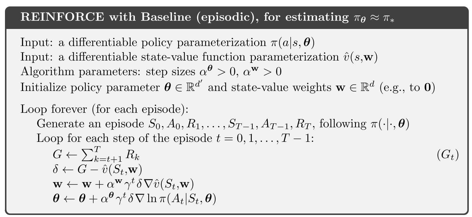
Monte-Carlo REINFORCE
Let’s start with the simplest Policy Gradient algorithm (Williams 92). I’m writing a simple PyTorch implementation of this algorithm using OpenAI’s Cart-Pole environment (Yes, another one). The full code is avaliable on my Github page.
Pseudocode
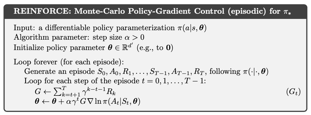
As you can see in the title this is an MC solution, we collect full episodes and update the model after each episode.
Let’s code our function approximator. We are going to use a simple architecture because of the simplicity of this environment (only one hidden layer with 128 neurons).
class MC_REINFORCE(nn.Module):

    def __init__(self, n_inputs, n_actions, n_hidden):
        super(MC_REINFORCE, self).__init__()
        self.actor = nn.Sequential(
            nn.Linear(n_inputs, n_hidden),
            nn.ReLU(),
            nn.Linear(n_hidden, n_actions)
        )


    def forward(self, state):
        norm_state = self._format(state)
        logits = self.actor(norm_state)
        probs = F.softmax(logits, dim=1)

        return probs


    @staticmethod
    def _format(state):
        if not isinstance(state, T.Tensor):
            state = T.tensor(state, dtype=T.float32)
            state = state.unsqueeze(0)
        return state


    def get_action(self, state):
        # Calc the probabilities
        probs = self.forward(state)

        m = Categorical(probs)
        action = m.sample()
        logprobs = m.log_prob(action).unsqueeze(-1)
        return action.item(), logprobs
In episodic environments it is not neccessery to calculate discounted rewards but practically it is more efficient, hence we are going to implement it. Formally:\(\sum_{t=0}^{T-1} G_t * \gamma^t\)
That summation looks scary with \(\gamma^t\) but actually it is pretty simple as you can see below in the code block.
def calc_returns(rewards, gamma):

    returns = list()
    cumulated_reward = 0

    for r_t in rewards[::-1]:
      cumulated_reward = r_t + (cumulated_reward * gamma)
      returns.append(cumulated_reward)

    return returns[::-1]
Let’s assume your agent reached rewards 6 times with the value of one [1,1,1,1,1,1] and the gamma is 0.99 then the discounted returns are [0.95, 0.96, 0.97, 0.98, 0.99, 1.]. As you can see we have bigger discount on the earlier steps and it makes sense because we can’t be sure how good was each step in the trajectory (except we know the last steps weren’t good because we lost the game). We calculate the cumulative values for each step: [5.85, 4.9, 3.94, 2.9701, 1.99, 1.0]. It’s maybe a bit ambiguous since we discounted the initial state value much more than the last step but because we cumulated the values it has much bigger value then the others. We did this because after that step the agent was able to do N other steps too, so we assume earlier steps were effective but we still don’t calculate with the full values because we don’t know the precise efficiency.
Let’s see the training loop. I’m writing the comments into the code block because it is more straightforward there.
def optimization(self, returns, log_probs_):
        # calculating the discounted cumulative returns
        cumulative_r = self.calc_returns(returns, self.gamma)

        # calculating the loss function
        loss = -T.cat([lp_ * r for lp_, r in zip(log_probs_, cumulative_r)]).sum()

        # We use Adam optimizer
        self.opti.zero_grad()
        # backpropagation
        loss.backward()
        self.opti.step()


def train(self, N_EPISODES):

        self.env.seed(self.seed)
        returns_episode = list()

        #  Iterating through the defined number of episodes
        for e in range(N_EPISODES):
            state       = self.env.reset()
            log_probs   = list()
            rewards     = list()

            # Agent makes action until reach the maximum steps in the environment or lose the game
            for _ in range(10000):
                # We calculate the probabilities and choose an action based on the probability distribution
                action, log_p = self.agent.get_action(state)
                # Step with the chosen action and collect the reward
                new_state, reward, done, _ = self.env.step(action)

                # We collect the log probabilities and the rewards per state since we calcualte the loss function with these values
                log_probs.append(log_p)
                rewards.append(reward)

                # If the agent reached a terminal state or maximized the steps then the game is over.
                if done:
                    break

                state = new_state

            # Optimizing the agent
            self.optimization(rewards, log_probs)
REINFORCE with Baseline (Vanilla Policy Gradient)
As I mentioned above REINFORCE has high variance (this baseline solution is also part of the original Williams’ paper) and this modification gonna reduce the variance but it is still unbiased.
How is it possible? We have to choose a value that is independent of our gradient: the value of the state, the average value of the rewards, or a moving average of the rewards. Then we subtract that value from \(G_t\).
For example, let’s assume on state s our agent chose an action a and this combination is part of two different trajectories. The value of G (cumulated reward) in the first trajectory is 50 while in the second one is “only” 23. We calculated the average reward in that state which is 25. Without the advantage function, we’d like to increase the probability of this certain action because the value of \(G\) is positive, but because we are using the advantage function in the first case the value of A is still quite high it is 25 (50 - 25 = 25) meanwhile in the second case it turns to be a negative value (23 - 25 = -2). CartPole is a good example for presenting this problem (environment only with positive rewards) but after this modification, our agent is able to learn from weaker trajectories.
Formally: (Advantage function)
\(A = \sum_{t=0}^{T-1} G_t * \gamma^t - b(s_t)\)
Pseudocode
If we are going to calculate the value of the states then we have to implement another neural network that will calculate those values in an on-policy way. Simple architecture as you can see in the code block below.
class SVN(nn.Module): # State-value network

    def __init__(self, n_inputs, n_hidden, n_actions=1):
        super(SVN, self).__init__()
        self.critic = nn.Sequential(
            nn.Linear(n_inputs, n_hidden),
            nn.ReLU(),
            nn.Linear(n_hidden, n_actions)
        )


    def forward(self, state):
        norm_state = self._format(state)
        state_value = self.critic(norm_state)

        return state_value


    @staticmethod
    def _format(state):
        if not isinstance(state, T.Tensor):
            state = T.tensor(state, dtype=T.float32)
            state = state.unsqueeze(0)
        return state
We also have to modify our optimization function since we use the advantage function.
def optimization(self, returns, log_probs_,  state_v):

        # We calculate the cumulative returns the same way as we calculate with REINFORCE
        cumulative_r = self.calc_returns(returns, self.gamma)

        # Transforming lists to tensors| state_v contains every statevalue per state of our trajectory
        cumulative_r = T.FloatTensor(cumulative_r).unsqueeze(1)
        state_v = T.cat(state_v)

        #  Calculate the value error
        value_err = cumulative_r - state_v

        # calculating the loss function | Instead of cumulative_r (returns) we use the value error values
        loss = -T.cat([lp_ * v for lp_, v in zip(log_probs_, value_err.detach())]).sum()

        # PN steps | we optimize first the  Policy network
        self.opti_ag.zero_grad()
        # backpropagation
        loss.backward()
        self.opti_ag.step()

        # SVN steps | then we optimize the state-value network
        self.opti_v.zero_grad()
        # As you can see here we calculate mean squared error value error^2 and backpropagate on the value  network
        value_loss = (value_err**2).sum()
        # backpropagation
        value_loss.backward()
        self.opti_v.step()
I also present a chunk from the train function, because it is important how we calculate the state values.
for _ in range(10000):
                # Same as REINFORCE
                action, log_p = self.agent.get_action(state)
                new_state, reward, done, _ = self.env.step(action)

                # Calculate state value |  We calculate the state value
                state_v = self.value_n(state)

                # Append to a list
                state_values.append(state_v)
                log_probs.append(log_p)
                rewards.append(reward)
The whole implementation is avaliable on my Github page
Settings:
- The number of episodes: 2000
- The value of gamma: 0.99
- Policy networks optimizer: Adam (Value network: RMSprop)
Let’s compare the results
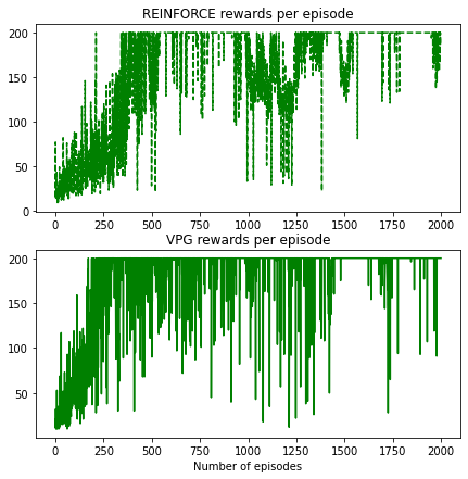
It looks a bit messy but I think you can see the differences. VPG reached faster the maximum reward of the environment (200) than REINFORCE. However, in this simple environment both approaches work well. There are huge drops on the chart thanks to the random steps, this is the way how the agent explores the environment. With time the optimization process improves the model performances and these drops are smaller and smaller because the probability of the good actions are higher every episode.
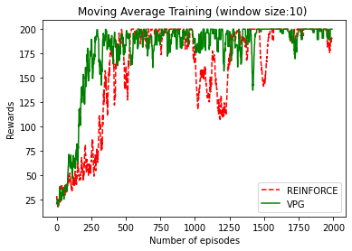
The visualization of the improvement is clearer if we follow the process on a chart where the rewards are adjusted with a simple moving average (in this case the window size is only 10).
I hope you found interesting this explanation of these state-of-art solutions, if you spotted any mistakes or you have any suggestions or you just want to chat then drop an e-mail to me.